How litopc corrects the mask.

New to lithography? Start with the plain-language guide.

The target is your intended printed shape.

The mask is the geometry that produces it through the optical model. Drawing those two shapes identically does not generally give an identical contour: neighboring features interact, line ends shorten, and corners round.

Optical proximity correction, or opc, deliberately biases the mask so the resulting contour follows the target more closely. litopc runs model-based opc, an edge-driven loop: it simulates the image, measures the error, moves the mask edges, then simulates again. The target stays fixed throughout. This is a local feedback method, not a neural network or a globally optimized inverse-lithography solver.

This replay uses the current correction code and optical engine.

Each displayed mask has been re-simulated, and the contour and error belong to that exact mask. Scrub the steps to see where the contour improves and where it still differs.

Before correction25.31 nm mean EPE

Iteration 00 / 1025.31 nm mean EPE

Recorded in litopcDUV 193 nmNA 0.93Threshold 0.3512² grid

Animated between recorded steps. EPE values are recorded results. Results depend on the pattern and settings.

The recorded run starts at 25.31 nm mean EPE and reaches 3.48 nm after 10 iterations, measured the way the simulator reports it: the target outline sampled every 18 nm against the printed contour. These values describe this example, not a general accuracy claim. Iteration 5 is slightly worse than iteration 4: correction is not guaranteed to improve at every step.

Settings: DUV dry, λ = 193 nm, NA = 0.93, σ = 0.7, threshold 0.3, best focus, 1100 nm field, 512² grid, 80 nm segmentation, gain 0.5, and 7 samples per exposed edge: the simulator's own defaults for this tool, with ten iterations instead of the three (Free) or five (Pro) of one batch.

litopc first resolves overlapping rectangles and splits long edges into segments.

Mask and target segments stay paired. Interior edges created by the split are excluded, so only the exposed boundary is measured.

For each sampled target point p_i, litopc finds the nearest point q_i on the simulated contour within a bounded search region. The displacement projected onto the target’s outward normal n_i is the signed edge placement error:

e_{i} = (𝒒_{i} - 𝒑_{i}) \cdot 𝒏_{i}

(1)

Scroll the diagram to see its full width.

Schematic, not to scale. The target stays fixed. Signed error tells each exposed mask edge which way to move.

Negative error means the contour is inside the target along that normal; positive error means it is outside. A bounded search helps avoid measuring an unrelated neighboring line. Missing contours or unmeasurable target edges stop correction; they are not counted as zero error.

Each iteration reports the mean and the largest absolute sample error. Mean EPE summarizes the boundary; maximum EPE marks the worst sampled location:

{EPE}_{mean} = \frac{1}{K} \sum_{i = 1}^{K} | e_{i} |, {EPE}_{\max} = \max_{i} | e_{i} |

(2)

K is the number of valid exposed-edge samples. These are sampled statistics, not a continuous worst-case bound over every point of the shape.

This per-edge measurement drives the correction. The figure the app reports, in the Correct card, the target score and every study, is a second, stricter rule: the whole target outline, corners included, sampled every 18 nm and matched to the nearest printed contour point. The two agree when the print is close; they differ at rounded corners and pulled-back line ends, which the per-edge samples deliberately skip (they start 15 % in from each corner). Reporting the outline figure keeps one definition of EPE across the product; the model guide states it as an equation.

CD measures feature width, not placement: the width can look reasonable while both edges are shifted. Check the spatial EPE overlay as well as the average, especially at corners and line ends.

Each exposed mask edge receives a proposed outward displacement Δb based on its mean signed error.

The gain g controls how much of that error to correct at once:

Δ b_{j} = - g {\bar{e}}_{j}

(3)

If an edge’s mean error is −10 nm and g = 0.5, its proposed mask growth is +5 nm before constraints. This does not predict a 5 nm contour movement: neighboring edges, diffraction, thresholding, and grid sampling couple the response. That is why the next optical simulation is essential.

The default is g = 0.5. Once two results are available, a rise of more than 2% in mean EPE reduces the gain for the next iteration by 25%, down to a floor of one quarter of the starting gain. A worse iteration stays in the history; it is not replaced by a better-looking result.

Every corrected mask is simulated and measured before it is shown, so N correction steps take N + 1 optical simulations including the baseline. Every frame in the replay follows that rule.

Proposed movements are constrained by minimum width, minimum space between distinct shapes, maximum edge bias, and grid snapping.

Interior edges stay fixed. These checks constrain the local updates; they are not a full mask rule check.

Enabled preset	Min. width / space	Max. bias	Grid
DUV dry	50 / 50 nm	80 nm	1 nm
EUV Low-NA	12 / 12 nm	20 nm	0.5 nm

Maximum bias is measured from each edge’s starting position for the current correction batch. Continuing in a new batch resets that reference; it is not a lifetime limit measured from the original design.

Correction requires a target built from rectangles. Fine segmentation reveals local error but can leave short edges unmeasurable; if a feature does not print at all, change the geometry or settings rather than trusting a low score.

Start with a built-in pattern such as an L-corner.

Simulate it and compare the target and contour. Run Correct, then inspect the verified history and EPE overlay. Look for missing features, narrowed connections, overshoot, or improvement concentrated on only one part of the boundary.

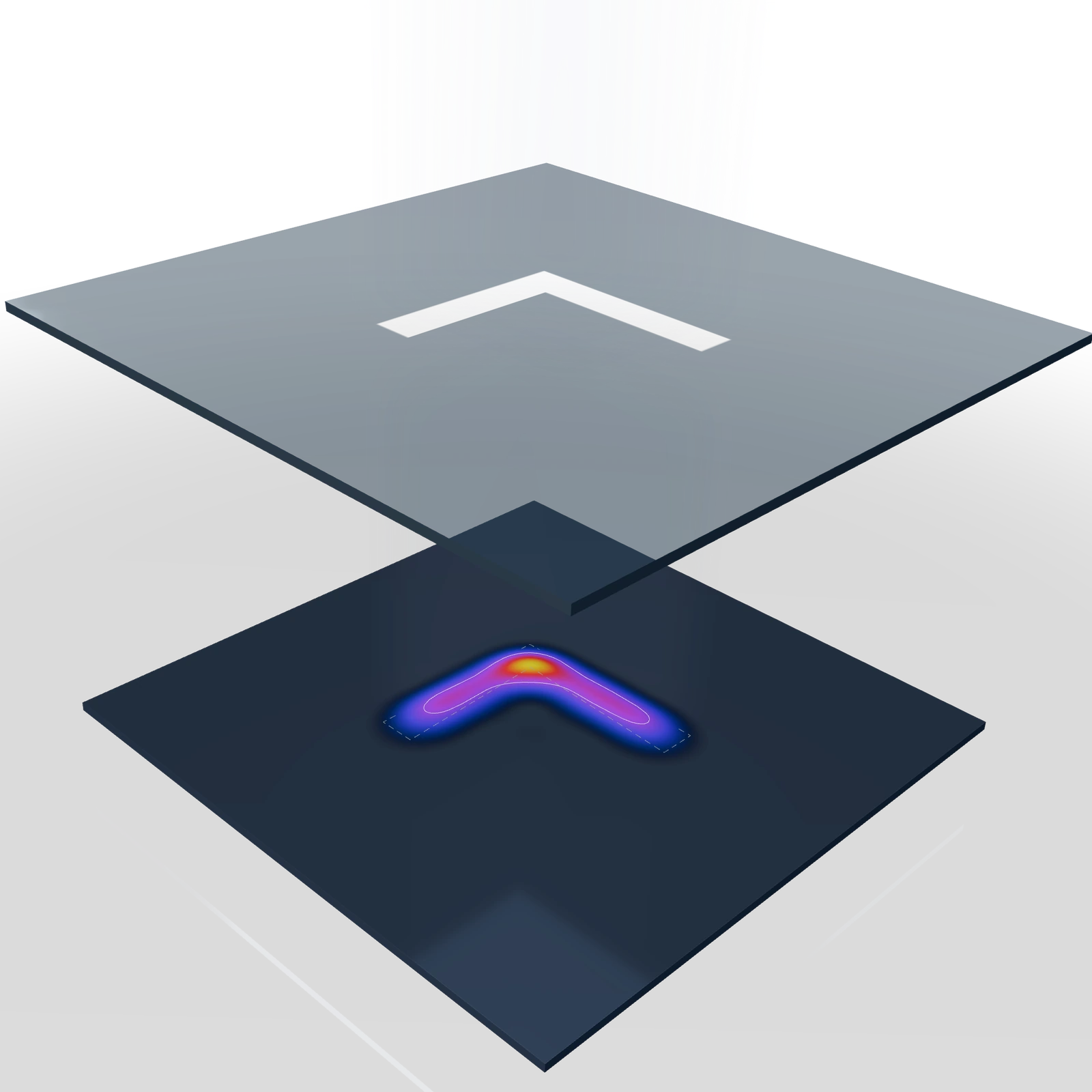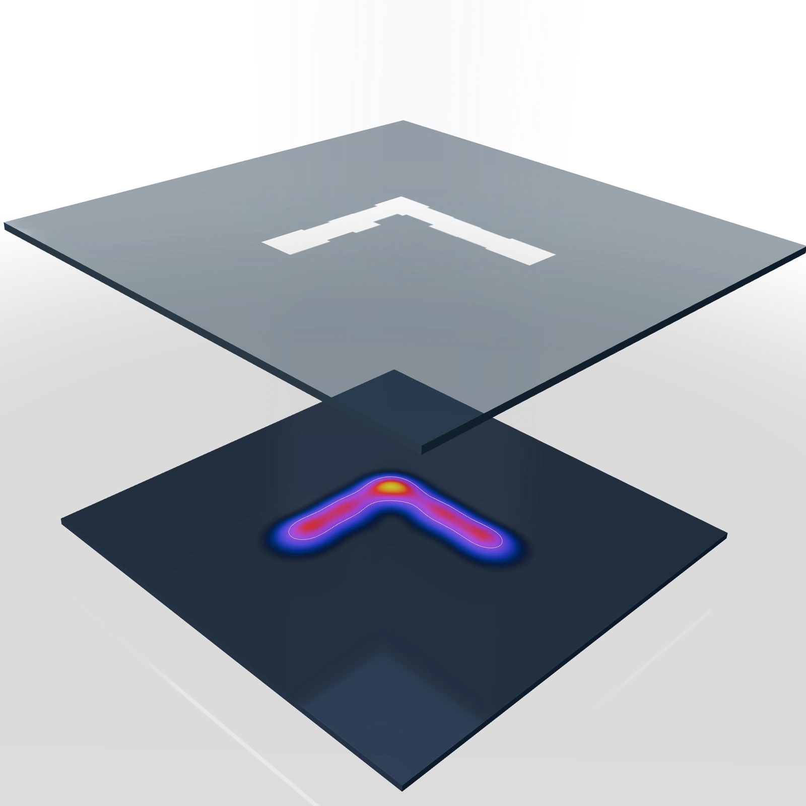litopc 3D view of the L-corner, before correction: the mask plate above, the light on the wafer below — litopc 3D view of the recorded L-corner run, before and after five iterations. The corrected mask grows small ears and notches, and the light on the wafer comes out fuller along the whole L.

litopc 3D view of the L-corner, after correction: the mask plate above, the light on the wafer below — litopc 3D view of the recorded L-corner run, before and after five iterations. The corrected mask grows small ears and notches, and the light on the wafer comes out fuller along the whole L.

Keep the optical preset, field, grid and threshold fixed when comparing correction steps. If you change those settings, evaluate the corrected mask again. A low error at one setting does not establish a process window or manufacturing robustness.

Use Apply to Mask to keep editing a result you have inspected, and export a 2D or 3D figure or the correction GIF to share the progression. For the assumptions behind the simulated contour, read the model simulation guide.

Open litopc simulator How the print is simulated

The target is not the mask.

One L-corner, ten corrections.

Edge placement error.

Moving mask edges.

Geometry constraints.

Read the shape, not just the score.